
Understanding the properties of permanent magnetic materials like Neodymium Iron Boron (NdFeB) is critical to their use in a variety of applications. These properties are typically quantified by four key parameters: remanence (Br), coercivity (Hcb), intrinsic coercivity (Hcj), and maximum energy product (BH(max)). To truly grasp these indicators, we need to understand the demagnetization curve – a tool that effectively reflects the overall performance of a magnet.
Understanding the properties of permanent magnetic materials like Neodymium Iron Boron (NdFeB) is critical to their use in a variety of applications. These properties are typically quantified by four key parameters: remanence (Br), coercivity (Hcb), intrinsic coercivity (Hcj), and maximum energy product (BH(max)). To truly grasp these indicators, we need to understand the demagnetization curve – a tool that effectively reflects the overall performance of a magnet.
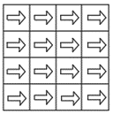
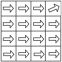
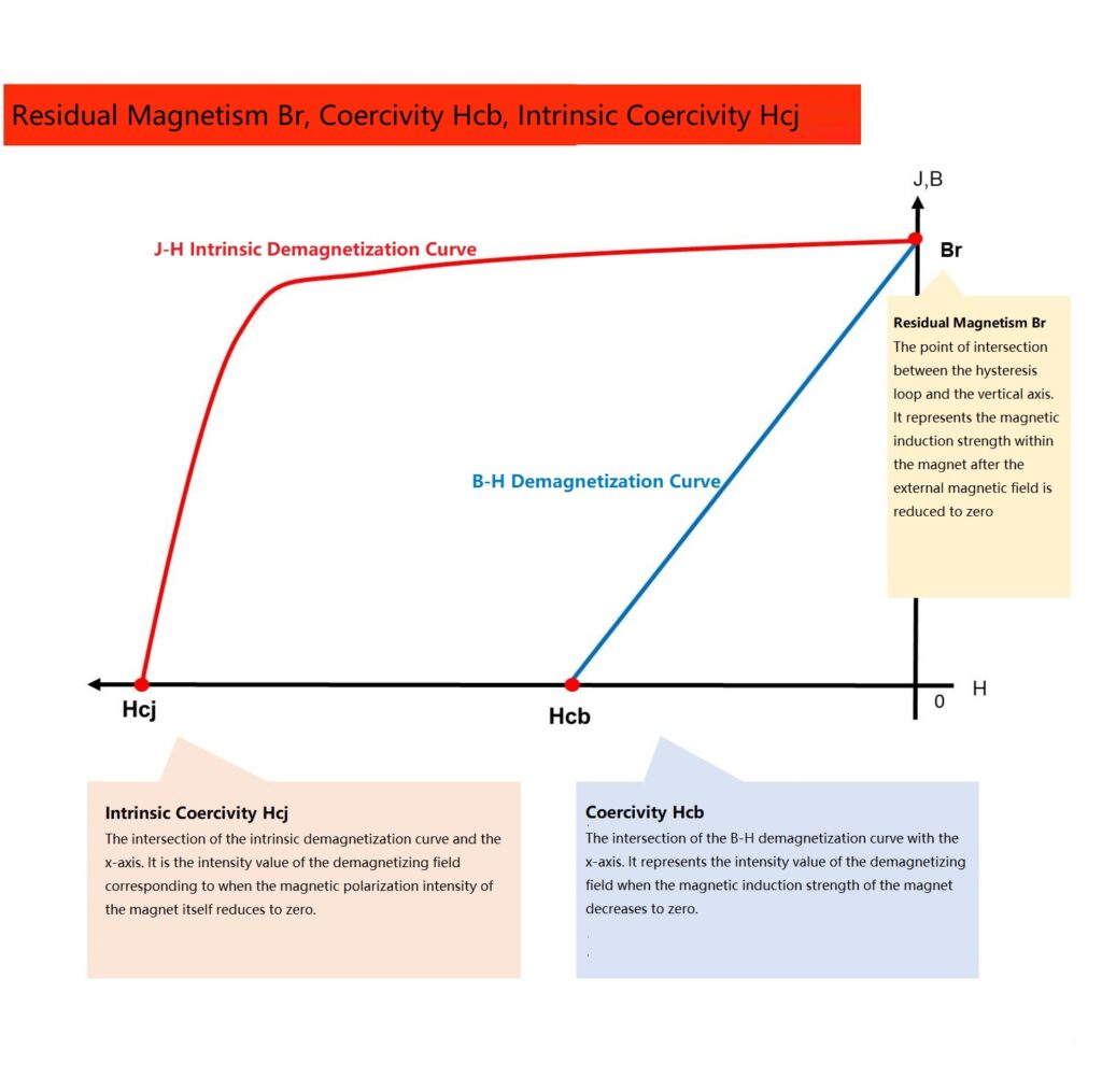
The four magnetic performance parameters of remanence, coercivity, intrinsic coercivity, and maximum energy product all originate from the demagnetization curve. In the above figure, the red line is called the J-H demagnetization curve (the change curve of magnetization strength J and external magnetic field H), also known as the intrinsic demagnetization curve. The blue line is called the B-H demagnetization curve (the change curve of magnetic induction strength B and external magnetic field H). We use small squares to represent individual magnetic domains, which can be understood as tiny magnets. A magnet is composed of a large number of magnetic domains, the arrows are the spontaneous magnetization direction C axis. For a magnetically neutral permanent magnet (simply understood as a magnet that has not been magnetized), most of the magnetic domains are in the same coordinate but cancel each other out in direction. In this way, no magnetism is exhibited externally, as shown in Figure 1.
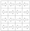
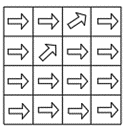
When a magnetic field is applied along the magnetization direction, the magnetic domains gradually align their C-axis direction through magnetic domain wall displacement and rotation, as shown in Figure 2 and Figure 3. This is the magnetization curve. The magnetization strength value of the magnet when fully magnetized is called saturation magnetization strength Js.
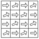
Next, let’s look at what happens when we take away the external magnetic field after the magnet is fully magnetized. According to Figures 4, we can see that most magnetic domains hold their direction steady, with a minor part exhibiting slight rotation. However, even in these cases, the primary direction remains the same. As a result, both the magnetic induction strength and the magnetization strength of the magnet continue to exhibit high values. We term this value as the residual magnetic induction strength (Br) or the residual magnetization strength (Jr). You can visualize this as the leftover magnetization of a magnet once the external field is no longer present. When the external magnetic field (H) is zero, Br equals Jr. We frequently use Br, also known as remanence, to describe this state, measured in either Gauss (Gs) or Tesla (T). The higher the Br, the stronger the retained magnetic induction strength, and the greater the potential to become a strong magnetic material.
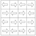
What if we apply an external magnetic field in the reverse direction? Our magnet’s magnetic domains start to displace and rotate, as depicted in Figure 5. Once the magnetic field strength hits a specific point, the magnetic induction strength (B) of the magnet falls to zero. In simpler terms, the magnet’s retained magnetic field strength is counteracted by the newly added reverse magnetic field strength. The corresponding magnetic field strength at this time is termed as the coercivity (Hcb, sometimes notated as bHc), measured in Oersteds (Oe) or kiloamperes per meter (kA/m). Hcb plays a vital role in the slope of the J-H demagnetization curve. If the displacement or rotation of the magnet’s magnetic domain is challenging within a short time, the J-H line will be almost straight. Consequently, the value of Hcb will approach Br indefinitely. The highest value Hcb can reach is Br. The ideal situation, Hcb equals Br, implies no magnetic domain reverses until the reverse magnetic field strength numerically matches Br. Therefore, the magnet is extremely stable, meaning it resists demagnetization effectively when the reverse magnetic field’s value is below Br.
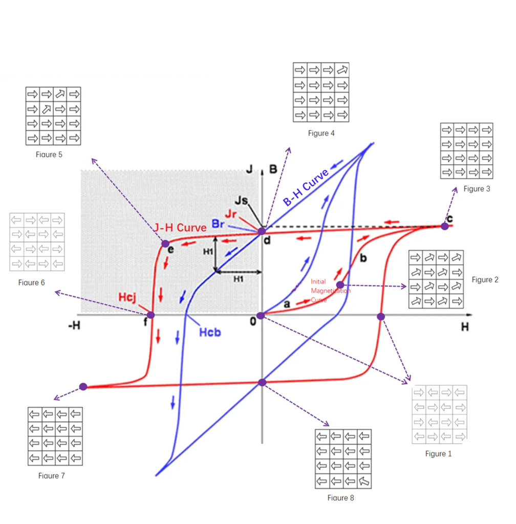
When we continue to increase the reverse magnetic field and it reaches a critical value, reverse magnetic domains appear quickly, causing the magnetization strength of the magnet to plummet to zero. Essentially, the retained magnetic field strength within the magnet drops to zero, as shown in Figure 6. The corresponding magnetic field strength value at this time is termed as intrinsic coercivity (Hcj, sometimes noted as jHc), measured in Oe or kA/m. Intrinsic coercivity is a measure of a magnet’s resistance to demagnetization. The larger the intrinsic coercivity, the stronger the resistance to demagnetization or, more precisely, the stronger the resistance to total demagnetization. It’s crucial here to understand the difference between Hcj and Hcb. If Hcj is greater than Br, Hcb’s limit is Br. If Hcj is less than Br, Hcb’s limit is Hcj.
On the demagnetization curve B-H, the product of B and H at any given point is known as magnetic energy product. The peak value of this product is the maximum energy product, (BH)max. In theory, (BH)max equals ½ Br². This maximum magnetic energy product balances remanence and magnetic coercivity. Its numerical value represents the size of the magnetic energy contained within the magnet, reflecting the initial slope of the J-H line. The units are usually given in GOe or j/m³.
If these four parameters still feel tricky to grasp, let’s put it simply: think of a magnet as a cup of water. Magnetizing the magnet is akin to heating the water. The remanence is the heat retained in the water after you stop heating, and demagnetization is similar to cooling the water down. Coercivity, Hcb, is like the ambient low temperature needed to neutralize the heat in the water, making it imperceptible from the outside. Intrinsic coercivity, Hcj, is equivalent to the ambient low temperature required to cool the water’s heat to zero. Below is a simplified graph of the second quadrant of the hysteresis loop to aid your understanding of these concepts.
For the above magnetic parameters, we should pay attention to the following points in practical applications:
- 1. For magnets that require a strong magnetic field, we usually need to increase their remanence as much as possible to release more magnetism. However, it should be noted that this is on the premise of no demagnetization. If demagnetization exists, simply increasing remanence may be ineffective. We also need to increase Hcj to reduce demagnetization. A simple example is a 0.5’’ dia x 0.375’’T disk-shaped magnet. The surface magnetism of 52H is higher than that of N52. The reason is that the Hcj of 52H is higher, allowing its Br to be fully utilized. The Hcj of N52 is very low, and it cannot maintain a state of no demagnetization. No matter how high the Br is, its magnetism cannot be fully utilized
- 2. For magnets that require resistance to demagnetization and high stability, we usually need to increase Hcj. In addition, we need the Hcb value to be as close to Br as possible
- 3. For magnets that require good temperature resistance, we usually choose to increase Hcj. Because the temperature coefficient of the coercivity of neodymium iron boron permanent magnets with the same Hcj is not much different, the most direct effect of increasing Hcj is to delay or prevent the turning point of the B-H line from appearing. If the temperature stability requirements are strict, we also need to consider the requirements of Hcb, try to reduce the slope of the B-H line, and reduce the irreversible decay amplitude of the magnet