
Overview
In the realm of energy conversion, linear and planar motors stand out as groundbreaking innovations. These devices, with their ability to effortlessly morph electrical impulses into linear mechanical actions, have redefined efficiency. By sidestepping the intricacies associated with intermediary conversion tools, they offer a streamlined and robust design. This design ethos translates into a host of benefits: a minimalist yet effective structure, rock-solid transmission stability, lightning-fast dynamic responses, and laser-sharp positioning capabilities. Such attributes have paved the way for their integration into a plethora of modern systems.
From state-of-the-art logistics frameworks and precision-driven CNC tools to the latest in lithographic methodologies and next-gen magnetically levitated transit modules, their influence is undeniable. Amidst these advancements, the 1D Halbach permanent magnet array emerges as a pivotal component. Crafted with a meticulous arrangement of permanent magnets, it radiates a potent magnetic aura on one flank. This aura, characterized by its rhythmic sinusoidal waves, accentuates the array’s adaptability, earmarking it as a top choice for diverse motor designs, be it linear or planar.
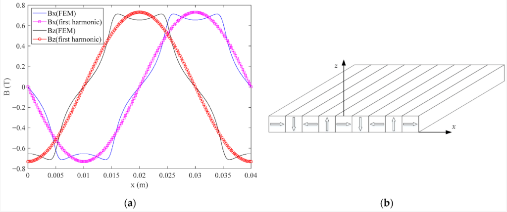
To further elucidate, Figure 1 (a) provides a visual representation of the first harmonic and FEM of magnetic flux density. Additionally, Figure 1 (b) offers a glimpse into the conventional magnet array with rectangular magnets, highlighting the stark contrasts and advantages of the Halbach design.
Unveiling the Design of the Advanced Magnet Array
In the quest to model magnetic flux density, an innovative magnet array emerges, drawing inspiration from the traditional array with rectangular magnets. The design of this permanent magnet aims to achieve an optimal sinusoidal magnetic field. The approach to this analysis is systematic. Initially, the permanent magnet is segmented into smaller units. Subsequently, each segment’s height is individually determined. Culminating the process, the magnetic flux density is extrapolated using the Fourier series.
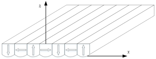
Figure 2 offers a visual perspective, revealing the magnet array’s cross-section and the \(Mx\) projection distribution for these segmented permanent magnets in the \(x\) magnetization direction. Arrows indicate the magnetization direction, flowing seamlessly from the S pole to the N pole. Each of these fragments mirrors a rectangular magnet, symbolized by the blue bar.
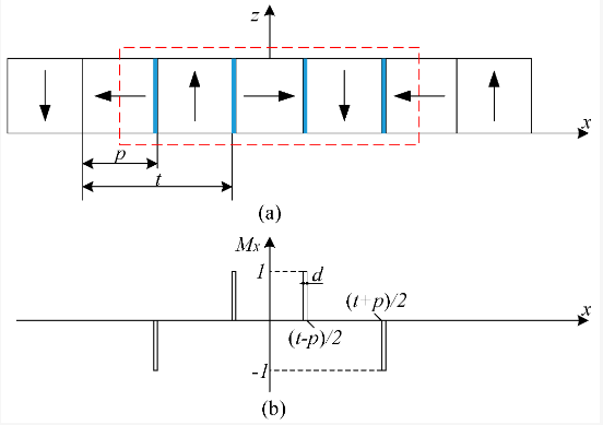
Building on the periodic and symmetrical attributes of the magnet array, all permanent magnets undergo segmentation into equal-sized pieces. Each segment shares identical side lengths. Every permanent magnet boasts a central axis of symmetry, flanked by symmetrical distributions on either side. Consequently, within a single period, four segments of equal heights emerge, collectively visualized as a group in Figure 2. If a permanent magnet is dissected into 2n pieces, with n being an integer, then half of that magnet comprises n pieces. This leads to the deduction that permanent magnets, when magnetized in the x-direction of the magnet array, are assembled from n groups of pieces. The same holds true for those magnetized in the z-direction.
The \(Mx\) component of the magnet array, rooted in the Fourier series, is articulated as:
\[Mx=M\sum_{k=1}^{\infty}\sum_{i=1}^{n}a(i,k)cos(k\omega x)\]
Here, various parameters come into play, such as \(M=\frac {Br}{\mu0}, \omega=\frac {\pi}{t}\), and so on.
Figure 3 illuminates the \(Mz\) projection distribution of the permanent magnets in the z magnetization direction.
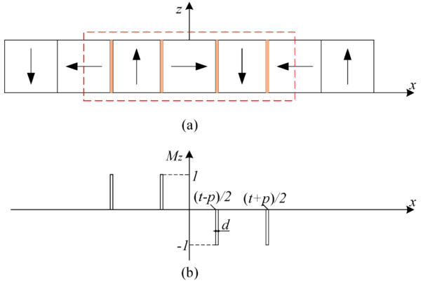
The magnet array’s magnetization vector is a blend of \(Mx\) and \(Mz\) components. The \(Mz\) component, too, finds its roots in the Fourier series. The expression for \(Mz\) is
\[Mz=M\sum_{k=1}^{\infty}\sum_{i=1}^{n}b(i,k)sin(k\omega x)\]
The magnet array’s magnetization vector is then deduced and expressed in a specific format, incorporating both \(Mx\) and \(Mz\) components.
The magnetic field’s spatial distribution encompasses three distinct regions: air, the permanent magnet array, and again, air. The magnetic scalar potential method is employed to decipher the magnetic flux density, given the absence of conduction current.
Boundary conditions at the interface are derived from Maxwell’s equations, simplifying the magnetic field problem to solving the Poisson equation of magnetic scalar potential. The magnetic flux density is then ascertained using the variable separation method, expressed in a specific format for the region beneath the magnet array.
Lastly, it’s imperative to note the assumption regarding the relative permeability for the permanent magnet µr, which is taken as 1.0. Given the utilization of high-caliber sintered NdFeB permanent magnets, any error stemming from this assumption is negligible.
Design of New Magnet Array
Refinement Process
The primary objective is to achieve a magnetic field that closely resembles a sinusoidal pattern. This ensures that the real magnetic flux density aligns with the primary harmonic of the magnetic flux density. Consequently, the real magnetic field exhibits strong sinusoidal traits, simplifying its representation to that of the primary harmonic.
In the dynamic control of electric machinery, the primary harmonic of the magnetic flux density is typically employed for force calculations. The novel magnet array is conceptualized based on the traditional array, with an emphasis on surface shape optimization. Hence, the primary harmonic of the magnetic flux density from the conventional array is the foundation for our optimization.
The optimization process focuses on minimizing the influence of higher harmonics. The shape of the curved surface is derived by adjusting the height of the smaller segments. Given that the horizontal thrust is a significant performance indicator for motors, the z component of the magnetic flux density, which produces this thrust, is the focal point of our objective.
For the traditional magnet array, the primary harmonic of the magnetic flux density can be deduced when n is set to 1, represented as:
\[\vec{B_1}=\begin{pmatrix}B_{x1} \\ B_{z1} \end{pmatrix}=-{\mu}_0 \omega K_1 e^{ws} \begin{pmatrix}cos(\omega x) \\ sin(\omega x) \end{pmatrix}\]
Here, \(B_{x1}\) and \(B_{z1}\) denote the primary harmonic of \(x\) and \(z\) components of the magnetic flux density.
From our objective function, it’s evident that reducing higher harmonics is a complex optimization challenge involving multiple variables. The Sequential Quadratic Programming (SQP) method, known for its convergence, computational efficiency, and robust boundary search capabilities, is employed for this optimization. To sidestep singular points and achieve superior optimization outcomes, we’ve determined that five segments for half of a single permanent magnet are optimal. This results in a total of 10 segments for the entire magnet, sufficiently showcasing the curvature of the magnet’s surface.
Tables 1 and 2 provide a detailed view of our optimization parameters and variables. Given the assembly dynamics of the permanent magnets, the top surface positions of each segment \((h_t(1), h_t(2), \cdots , h_t(5))\) are consistent. The variables for optimization are the bottom surface positions for each segment of half of a single permanent magnet \((h_p(1), h_p(2), \cdots , h_p(5))\).
Table 2’s “constraints” section outlines the optimization variable range. As the constraints for these five optimization variables are consistent, they’re represented as \(h_p(1) \sim h_p(5)\). Taking into account the optimization parameters, the upper limit for optimization variables doesn’t surpass the top surface position of the segments, i.e., 10 mm. Similarly, the lower limit doesn’t go beyond the objective region’s position, i.e., −2 mm.
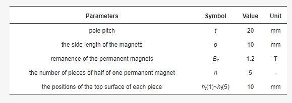
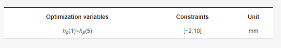
Figure 4 showcases the results, highlighting the minimization of the objective function. In this figure, the ‘current point’ signifies the best-found value of the optimization variables during the solver’s run. The ‘current function value’ represents the objective function’s value at this point.
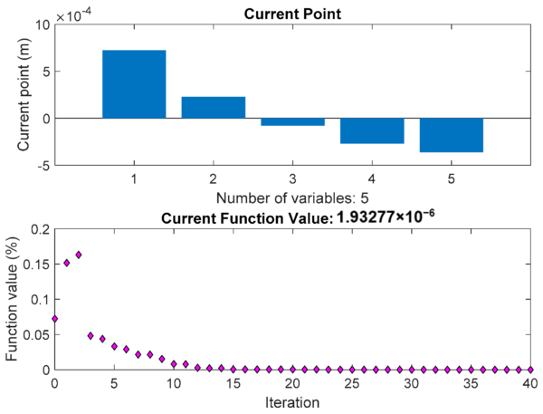
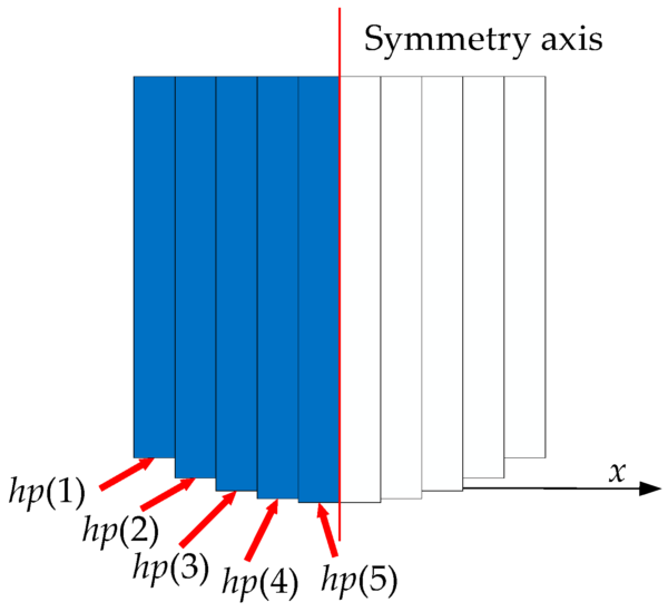
Figure 5 displays the segments of a single permanent magnet based on the optimization variables. In this novel magnet array, the optimized curved surfaces for the x and z magnetization directions are identical. The curved surface’s symmetry axis is centrally located, with both sides exhibiting a symmetrical pattern. The variables \(h_p(1) \sim h_p(5)\) are not only optimization variables but also represent the bottom surface positions of the segments for half of a single permanent magnet. Hence, the segments for a single permanent magnet can be deduced based on symmetry.
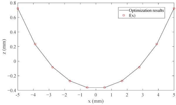
Taking a permanent magnet with its x-coordinate center at zero as an example, Figure 6 illustrates the optimized curved surface. The data forming this curved surface shape is derived from the optimization findings. The shape appears to follow a sine or power function pattern. We employed the least squares polynomial fitting to align the data. After comparing polynomials of degrees 2, 3, and 4, the fourth-degree polynomial emerged as the most precise. For clarity and without compromising accuracy, terms with negligible coefficients (first and third order) were omitted, resulting in a sum of squares due to error (SSE) of \(1.376 \times 10^{−10}m^2\). Figure 6 also presents the computed polynomial data, represented as:
\[f(x)=a_1x^4+a_2x^2+a_3\]
Here, \(a_1= 3.763 \times 10^5, a_2= 34.28\), and \(a_3= −3.699 \times 10^{-4}\) are the coefficients, with x’s value range being [−p/2, p/2].
Authenticating the New Magnet Array Using Finite Element Analysis
The innovative magnet array, characterized by its distinct curved surface, is visualized in Figure 7, derived from the results of our optimization process. To validate the efficacy of the optimization, we juxtaposed the magnetic flux density at varying z coordinates with the data generated from a finite element model (FEM). This FEM was meticulously constructed and analyzed using the renowned Ansoft Maxwell software, known for its precision-driven adaptive subdivision capabilities and its robust post-processing features.
The magnetic flux density, as determined by both the FEM and our analytical model, is depicted in Figure 8. The data reveals a remarkably sinusoidal pattern for the magnetic flux density. Impressively, the outcomes from our analytical model align closely with those from the FEM. To quantify the accuracy of the magnetic flux density, we employed the total harmonic distortion (THD) metric. The discrepancies between the analytical model and FEM, as well as the THD of the magnetic flux density, are tabulated in Table 3.
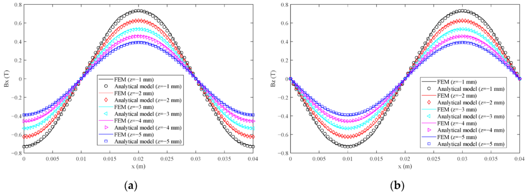
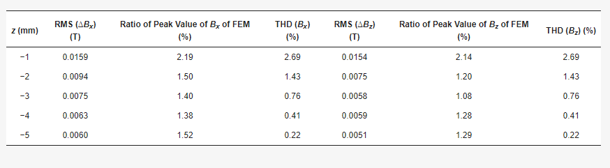
For different z coordinates, the values for RMS(∆Bx), RMS(∆Bz), THD(Bx), and THD(Bz) are minimal. The highest discrepancies for RMS(∆Bx) and RMS(∆Bz) are observed when z is at −1 mm, accounting for 2.19% and 2.14% of the peak values of Bx and Bz from the FEM, respectively. Both THD(Bx) and THD(Bz) values, as per the equation below, are identical. Their peak values, again at z = −1 mm, stand at 2.69%. Consequently, we’ve successfully crafted a novel permanent magnet array that boasts a pristine sinusoidal magnetic field, complemented by a straightforward analytical model for magnetic flux density.
\[\vec B=\begin{pmatrix}B_x \\ B_z \end{pmatrix}=-{\mu}_0 \omega \sum_{k=1}^{\infty} Ke^{\lambda z}k \begin{pmatrix} cos(k\omega x) \\ sin(k\omega x) \end{pmatrix}\]
Discussion
Varying Lengths of the Permanent Magnet
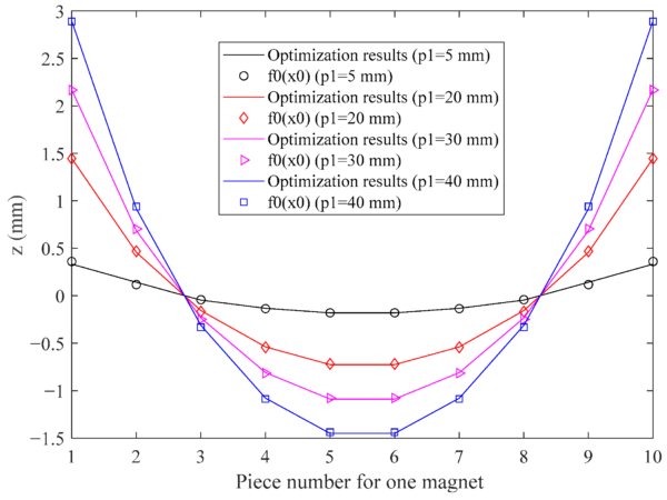
In this subsection, we delve into the adaptability of our optimized outcomes when there are alterations in the dimensions of the permanent magnet. The optimization insights were derived based on specific parameters of the magnet array. To cater to varying dimensions of the magnet, the fitting formula needs refinement. The updated expression is presented as:
\[f_0(x_0)=(a_1 x_0^4+a_2 x_0^2+a_3)\frac {p_1}{p}\]
Here, \(p_1\) represents the side length of the newly magnetized magnets in the \(z\) and \(x\) orientations. \(x_1\) is the updated \(x\) coordinate, confined within the range \(\left[ -p_1/2, p_1/2 \right]\).
For validation purposes, we consider \(p_1\) values of 5 mm, 20 mm, 30 mm, and 40 mm. Figure 9 illustrates the comparison between the optimization outcomes and the computed data from the revised fitting formula. The consistency observed between the two confirms the versatility of the new fitting expression, making it apt for magnets with diverse side lengths.
Varying Elevations of the Permanent Magnet
Our optimization insights are further validated by examining magnet arrays with diverse magnet lengths and elevations. This flexibility in design ensures that as long as the contour of the magnet’s bottom surface aligns with our optimization findings, we can achieve the targeted magnetic field intensity. By merely adjusting the magnet’s dimensions, the magnetic field retains its desirable sinusoidal attributes.
When delving into the height variations of the magnet, we juxtaposed the magnetic flux density from our analytical model with that of the FEM, particularly when ht(i) (where i=1,2,…,5) is designated as 5 mm and 15 mm. This comparison is vividly depicted in Figures 10 and 11.
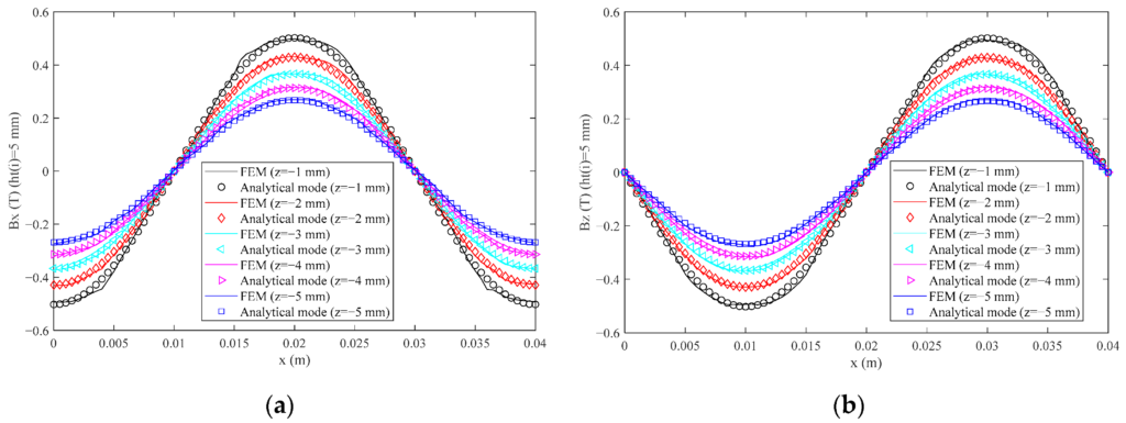
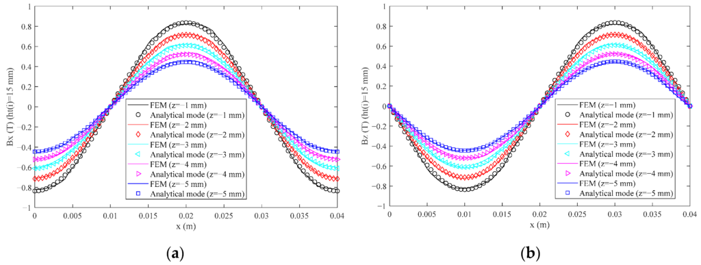
Figures 10 and 11 reveal that the magnetic flux density consistently showcases an impressive sinusoidal waveform. The analytical model’s outcomes are in harmony with the FEM’s findings. For instance, when ht(i) (where i=1,2,…,5) is set at 5 mm, the peak RMS(ΔBx) and RMS(ΔBz) values register at 0.0151 T and 0.0139 T, respectively. These figures represent 3.03% and 2.78% of the FEM’s Bx and Bz peak values. When adjusting ht(i) to 15 mm, the RMS(ΔBx) and RMS(ΔBz) values peak at 0.0183 T and 0.0168 T, respectively, equivalent to 2.22% and 2.06% of the FEM’s peak values for Bx and Bz. The maximum THD(Bx) and THD(Bz) values are observed when z is set to -1 mm, amounting to 3.53% and 2.37% of the peak value for heights of 5 mm and 15 mm, respectively. This underscores the adaptability of our new fitting expression to magnets with varied elevations.
Impact on Weight
In our innovative magnet array design, the permanent magnet’s cross-sectional shape deviates from the traditional rectangular form due to the introduction of a curved surface. It’s crucial to assess how this alteration influences the overall weight. To determine the total weight, we can aggregate the weights of all individual permanent magnets. Given the assumption that all permanent magnets are identical, we can gauge the weight impact by examining just one of them. By scrutinizing the permanent magnet’s cross-section, we can deduce the weight variation by integrating the function \(f_0(x_0)\) A positive outcome indicates a weight reduction, while a negative one suggests an increase. The integral is represented as:
\[I_{f0}=\int_{\frac {p_1}{2}}^{-\frac {p_1}{2}}f_0(x_0)dx_0=\frac {3a_1p^4+20a_2p^2+240a_3}{240p}\]
Next, we analyze the cross-sectional area ratio between the newly designed permanent magnet and the conventional rectangular one. The latter’s cross-sectional area is defined as:
\[A_c=p_1 \times khp_1=khp_1^2\]
Where \(khp_1\) denotes the cross-section’s height, with \(kh\) being the coefficient.
The derived ratio is:
\[R_m=\frac {I_{f0}}{A_c} \times 100\]
Interestingly, this ratio remains unaffected by the parameter \(p_1\). With the surface design setting p at 10 mm, the ratio remains constant for a given \(kh\). For instance, with \(kh=1\), the ratio stands at -0.372%. This slight increment barely influences the weight.
Impact of the Air Gap
The unique curved design of the permanent magnets means that the base of the new magnet array isn’t entirely flat. Some parts of this curved base dip below the x-axis, as indicated by our optimization findings. When compared to the traditional magnet array, the actual gap between the magnet and the coil is slightly reduced. This change in gap can affect the magnetic field strength if the gap remains consistent with that of the conventional array. Let’s delve deeper into how this curved design influences the air gap.
The deepest point of the curved design is achieved when \(x_0\) is at 0 mm in the function \(f_0(x_0)\). To maintain a consistent air gap, the new \(z\) coordinate value, where we measure the magnetic flux density, is:
\[z=z_0+f_0(x_0=0)=z_0+\frac{a_3p_1}{p}\]
Here, \(z_0\) represents the original coordinate value, which could be values like −1 mm, −2 mm, and so on.
The magnetic flux density has a direct relationship with the expression \(e^{(\omega z)}\) as per our earlier equation. The proportion of the magnetic flux density calculated at this new \(z\) coordinate to the original is:
\[R_z=\frac{e^{\omega _1z}}{e^{\omega _1z_0}} \times 100\]
In this context, \({\omega}_1\) is redefined for varying side lengths of the permanent magnet as:
\[{\omega}_1=\frac{\pi}{2p_1}\]
Interestingly, this ratio remains constant and doesn’t depend on the parameter \(p_1\), equating to \(e^{(\pi/2/p\times a_3)}\). For different magnet lengths, this value stands at 94.36%.
Taking the air gap into account, there’s a slight reduction in the magnetic flux density. This implies that our new magnet array, even with its unique design, can produce a robust sinusoidal magnetic field within a minimal air gap. This minor trade-off in magnetic flux density makes it particularly apt for precision tools that demand a tight air gap.
Influence on Force Dynamics
When assessing the force dynamics of our novel magnet array, it’s essential to juxtapose its force and force ripple against those of the traditional magnet array. In the real-time control analytical model, the magnetic flux density expressions for both magnet arrays are congruent.
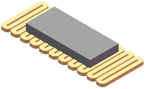
Taking a linear motor equipped with the innovative magnet array and coils as a reference, we can visualize its axonometric representation. This motor’s design, when integrated with the conventional magnet array, bears a striking resemblance, though no specific visual representation is provided here.
To simplify our understanding, let’s consider the motor’s cross-section when paired with both the new and conventional magnet arrays. The goal here is to eradicate any position-based discrepancies and ensure a consistent force across the array. This is achieved using the dq0 transformation combined with a three-phase coil.
Leveraging the magnetic flux density, the Lorentz force acting on the magnet array from a single coil can be determined through volume integral calculations. This force can be represented as a product of certain constants, the number of coils, and an exponential factor related to the coil’s position.
In conclusion, after thorough analysis and discussions, we’ve successfully developed a magnet array that produces a sinusoidal magnetic field. The optimized curved surface is versatile and can adapt to various permanent magnet dimensions. This flexibility in design ensures that, compared to its traditional counterpart, our new magnet array has a negligible impact on both mass and air gap. More importantly, it offers a significant reduction in force ripple, ensuring consistent performance even in smaller air gaps.
This study introduces an innovative 1D Halbach magnet array characterized by a uniquely contoured surface of the permanent magnet. Leveraging the superposition principle, we’ve devised a method to shape the magnet’s surface. This optimized contour closely resembles sine or power functions and can be represented using polynomial fitting. The magnetic flux density expression is straightforward, mirroring the first harmonic observed in the traditional magnet array with rectangular magnets. Notably, an optimal sinusoidal magnetic field emerges within an extremely narrow air gap. The optimization outcomes are versatile, accommodating various permanent magnet sizes. The magnet array’s weight impact is minimal. When the air gap is consistent with the traditional magnet array, there’s a slight dip in magnetic flux density. However, when compared to its conventional counterpart, our new magnet array drastically diminishes force ripple. This makes it an ideal choice for precision-driven devices that demand a minimal air gap. This magnet surface design approach can also be adapted for analogous 2D magnet arrays.