
Introduction
Magnetic fields, though invisible and intangible, play a vital role in numerous technological applications. Understanding their shape and direction can be challenging. Finite Element Analysis (FEA) serves as a powerful tool to demystify these enigmatic fields, providing a window into their behavior and interactions.
FEA Simulation: A Computational Approach
FEA, also known as FEA simulation, uses computer algorithms to simulate real physical systems through complex mathematical equations and models. By breaking down a system into simpler, interacting elements, FEA approximates a real system with a finite set of variables. This technique has widespread applications in fields like temperature, electric fields, magnetic fields, force fields, seepage fields, and acoustic fields. Popular magnetic field simulation software includes ANSYS, ABAQUS, Comsol Multiphysics, and JMAG-Designer
Mastering FEA software involves overcoming new software learning curves and understanding the magnetic parameters of various materials in the software’s material library. The magnetic field simulation is a specialized niche, and often, the software’s material library does not comprehensively cover all permanent and soft magnetic materials. This gap necessitates the creation of new materials and understanding their magnetic properties and demagnetization curves, demanding a thorough grasp of both material science and magnetic principles.
Typical Steps in FEA Simulation with ANSYS
Here’s a walkthrough of the standard steps in simulating the magnetic field of a permanent magnet using ANSYS software:
- Selecting the Design Type in FEA Software: Choosing the correct design module in FEA software is crucial for accurate magnetic behavior modeling. For magnetic field simulations, the static magnetic field module in software like ANSYS is typically the most appropriate choice. This module is specifically tailored to capture the nuances of magnetic field interactions in various applications.
- Modeling in FEA: Modeling begins with creating a precise representation of the magnet, including its geometry, positioning, and key attributes. Importing 2D and 3D models from drawing software into the FEA platform lays the foundation for a realistic and accurate simulation.
- Adding Material Properties: Defining the magnetic properties of materials is a pivotal step in FEA. For permanent magnets, accurately specifying the magnetization direction, typically in alignment with the coordinate system, is essential. This step requires in-depth knowledge of the material’s inherent magnetic characteristics.
- Setting the Computation Domain: The computation domain must be thoughtfully established to minimize errors and computational load. A well-chosen domain mirrors the actual environmental conditions surrounding the magnet, while keeping the computational requirements manageable.
- Boundary Conditions: Appropriate boundary conditions are vital for reducing the complexity of simulations and saving computational resources. In static magnetic field simulations, implementing ‘balloon’ boundaries is a common approach.
- The Excitation Source: For permanent magnet simulations, the magnetostatic static magnetic excitation is automatically selected in the software. When simulating coil magnetic fields, the excitation sources are typically voltage or current inputs.
- Grid Division: A critical aspect of FEA is the grid division, which connects finite elements to create a structural mesh. Finer grids provide more detailed results but require greater computational power.
- Solution Settings: In this step, error thresholds and computational steps are defined. Software like ANSYS often offers default settings that are optimized for a variety of scenarios.
- Performing the Solution Operation: This step involves running the simulation to achieve desired outcomes, such as visualizing magnetic field lines or obtaining quantitative field data.
- Post-Processing: Post-processing allows for the analysis of various outputs like magnetic field lines, cloud diagrams, and other simulated data. This step is crucial for interpreting the results and applying them to real-world scenarios.
Visualizing Magnetic Fields Through Simulation
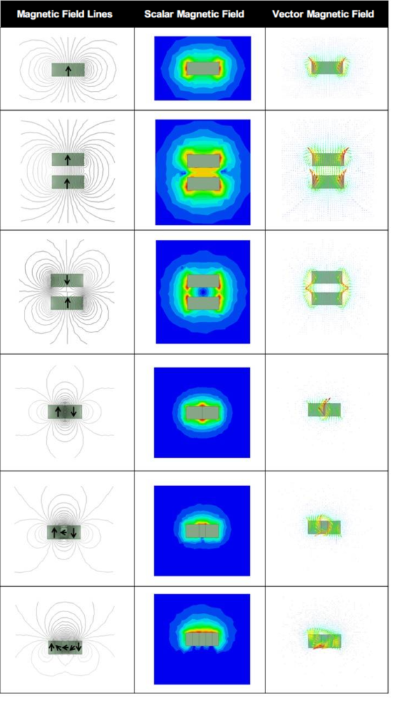
Having outlined the steps of using simulation software, let us now explore some magnetic field simulation images. These visualizations aid in understanding the distribution of magnetic fields in different magnetic circuits. They serve as a valuable tool in comprehending the complexities of magnetic interactions in various applications.
Conclusion: FEA as a Window to Magnetic Realms
FEA simulation provides an unparalleled insight into the distribution of magnetic fields in different magnetic circuits. By simulating these fields, engineers and scientists can design and optimize magnetic systems more effectively, paving the way for advancements in various technological fields.